How To Draw A Marginal Revenue Curve

It is now time to develop some technical concepts that will be useful in later assay. The first of these is the concept of elasticity. Until now we take described the shapes of demand and supply curves in terms of their slopes. It is not ever meaningful to describe curves as flat or steep, because whether a curve appears flat or steep depends upon the units in which price and quantity are measured.

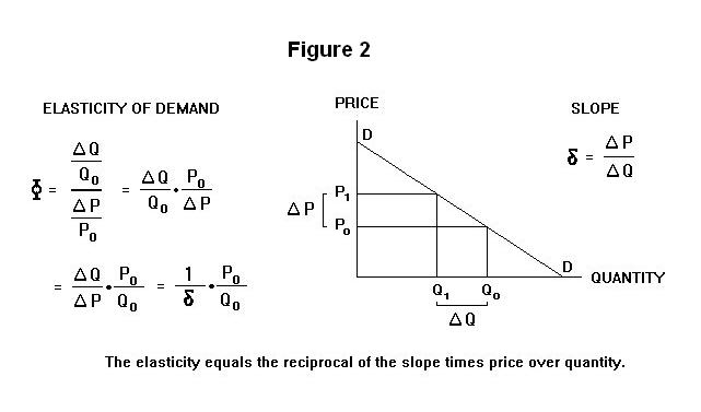
The gradient of the demand curve is shown in Figure ane. Permit  Δ  represent the words "small change". We tin can and then express the gradient of the demand bend, denoted by the greek symbol  δ,  every bit

Measure out the quantity of eggs in dozens and the toll of eggs in dollars. If, say, a rise in price of $1.00 reduces egg consumption by 5 dozen equally we motility up along the demand curve, the slope volition be -0.2.

At present suppose that we mensurate the quantity in numbers of eggs and the toll in dollars as before. The same demand curve volition now be flatter---a rise in the price of $1.00 volition reduce egg consumption by 60 eggs, yielding a gradient equal to -0.016667. If, alternatively, we were to mensurate the price of eggs in cents and the quantity of eggs in dozens, the slope of this aforementioned need curve would then be -100/five = -20. The apparent slope of the line on the graph will depend likewise on how widely we space the units of price and quantity along the axes---if, for example, the quantity units are spaced a quarter of an inch apart the bend will appear steeper than if they are spaced one-half an inch apart.

Past measuring the responsiveness of quantity to changes in toll using the concept of elasticity, we avert this dependence on units of measurement. The elasticity of demand is defined every bit the relative change (or percentage change) in quantity divided past the relative (or percentage) change in cost. Let united states use the greek symbol  Φ  to denote the elasticity of demand. Then we can write

2.       Φ  = ( ΔQ / Q ) / ( ΔP / P )

Since dividing past a number is equivalent to multiplying by its reciprocal we tin rewrite the above equation as

3.       Φ  = ( ΔQ / Q ) ( P / ΔP )   = ( ΔQ / ΔP ) ( P / Q )

Since the slope of the demand curve is equal to the alter in toll divided past the change in quantity, the term ( ΔQ / ΔP ) in the higher up equation is the reciprocal of the slope. Then we can write Equation 3 as

4.       Φ  = ( ΔQ / ΔP )( P / Q )   = ( i / δ )( P / Q )

The elasticity is the reciprocal of the slope multiplied by the ratio of price over quantity. All this is illustrated in Effigy ii where the elasticity of demand is measured relative to the initial price-quantity combination  ( P₀,Q₀ ) . It turns out that the elasticity will not be abiding as we movement along the curve. As should be articulate from Equation iv, given a constant gradient, the elasticity will decline as  P / Q  declines as we move down to the right along the straight-line need curve---at the vertical centrality where  Q  is zero the elasticity is infinite and at the quantity axis where  P  is cipher the elasticity is cipher.

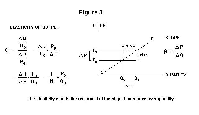
As shown in Effigy 3 below, the elasticity of supply is calculated in exactly the aforementioned mode every bit the elasticity of demand---the only divergence is that the elasticity of supply is positive while the elasticity of demand is negative, reflecting the fact that the supply curve is up sloping and the demand curve negatively sloped. Nosotros denote the slope of the supply bend by  θ  in the figure and mensurate the elasticity relative to the initial cost-quantity combination  ( P₀ , Q₀ ) . The elasticity volition non exist abiding as we movement up forth a straight-line supply curve unless that line passes through the origin, in which instance both the gradient and the ratio  P / Q  volition exist constant.

The total acquirement to the seller of a article, or total expenditure by the purchaser, is obtained by multiplying the price by the quantity. It appears in Figure 4 as the expanse of a rectangle whose bottom left corner is the origin and meridian correct corner is a point on the demand curve. The top left and bottom right corners equal toll and quantity respectively. The shaded rectangle in Figure 4, for example, gives the total revenue at signalc  on the demand curve---the production of the price  P₀  and the quantity  Q₀.  The full acquirement at pointa  is the rectangle  P_i a Q₁ 0.

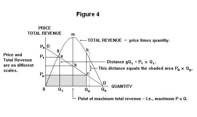
It is also clear in the above Figure that the full acquirement varies as we move forth the demand curve. The total revenue at zero quantity and price  P_m  is goose egg. As we motility down along the demand curve, the full revenue increases, reaching its maximum at the pointb  (which is centre-distant from the two ends of the curve) and and then declines, reaching null again at cost zero and quantity  Q_yard.

Total revenue is portrayed in the Effigy as the inverted parabola0 one thousand k h Q_k ---it is measured on a unlike scale on the vertical axis, of form, than is the price. The shaded expanse  P₀ c Q₀ 0  is equal to the distanceh Q₀.  Similarly, the area of the rectangle under the demand bend at pointb  equals the perpendicular distance betweenm  and the horizontal centrality. And the area of the rectangle under the demand curve at betokena  equals the distancethou Q₁.

Marginal revenue is defined as the change in total revenue that occurs when we modify the quantity by one unit. We can express the marginal acquirement, denoted by  MR,  as

5.       MR  =  ΔTR / ΔQ

where  TR  is total revenue. The marginal revenue is thus the slope of the total revenue curve in Figure five. At quantity zero, the marginal revenue is equal to the price---selling the get-go unit adds one times the price of that unit to the total revenue. Every bit quantity increases the marginal revenue falls because as we add successive units not only is the price of the terminal unit of measurement lower than the price of the previous unit simply all previous units accept to be sold at this lower toll.

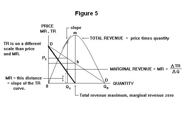
Marginal revenue for each quantity sold is given in Figure 5 every bit the altitude betwixt the thick line and the horizontal axis at that quantity. This distance is equal to the slope of the total acquirement curve at that quantity. At the bespeak of maximum total revenuethousand  the slope of the total revenue curve is cipher and the marginal revenue is therefore too zip. The marginal revenue curve thus crosses the horizontal axis at the quantity at which the total revenue is maximum. When the demand curve is a straight line, this occurs at the middle point of the curve, at a point on the horizontal axis that bisects the distance0 Q_k. Past the mid-bespeak of a straight line demand curve, the marginal revenue becomes negative.

Why is marginal revenue of import? This question is best answered past way of example. Consider the market for fresh eggs in a locality. Suppose that the government permits producers to establish an Egg Marketing Board with the power to set the price of eggs to the consumer and allocate output quantities to all individual producers. Purchases of eggs from outside the local expanse are prohibited. This state of affairs is shown in Figure 6. The demand bend is given by the line  DD  and the supply curve is the horizontal line  C₀S.  A horizontal supply curve is a reasonable assumption here because nearly of the inputs used to produce eggs tin exist purchased by egg producers at fixed market prices---these inputs are used past other industries and producers of eggs use a small fraction of the available supply. This implies that chicks can be hatched and raised to hens at constant toll.

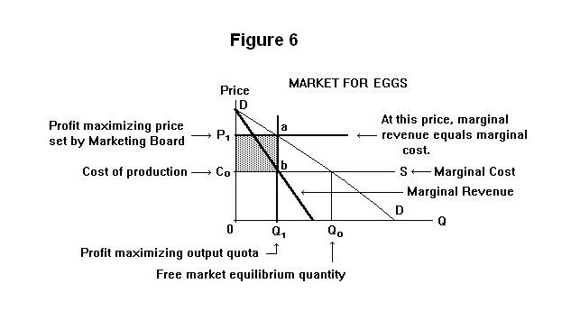
Egg producers like this organization because it enables them to sell their eggs to consumers at a price higher up the toll of production, yielding a turn a profit indicated by the shaded expanse in Figure six. The trouble faced past the Marketing Lath, acting on their behalf, is to determine the quantity level that will maximize that profit. At a lower output quota at that place is a gain from a higher cost, only the quantity producers sell will be less.

The profit is the excess of total revenue, given by the surface area  P₁ a Q_i 0,  over total cost, given by the area  C₀ b Q₁0.  At every quota level the Board's problem is to determine whether to increment the output quota past 1 unit of measurement. It will practise this if the additional revenue from selling another unit of measurement to consumers---the marginal revenue---is greater than the additional to total toll from producing another unit---called the marginal price.

The marginal revenue is given by the thick line in Effigy 6. The marginal price is given but by the horizontal supply curve---each additional unit produced adds0 C₀  to total cost. Starting from zero, therefore, the Board will increase the quota, unit by unit, until the marginal revenue curve crosses the marginal cost curve (in this case, supply bend). Output will expand until marginal revenue equals marginal cost. At this output level the profit to egg producers will be maximized.

If, starting from the output  Q₁ in Figure 6, the Board were to increment the output quota past i more than unit, the increase in total revenue from selling that unit would be less than the increase in the total cost from producing it, making such an expansion of the quota non worthwhile. Alternatively, if it were to reduce the quota past one unit, the reduction in total revenue from selling one less unit would be greater than the reduction in the total cost from producing one unit less, making the reduction in the quota not worthwhile. Profits are maximized by adjusting the quantity sold to equalize marginal cost and marginal revenue.

Economists have a convention of referring to the elasticity of demand as positive number even though it is in fact negative. When they talk virtually an elasticity of demand greater than ane they really mean that the elasticity of demand is less than -1. What they are referring to is the accented value of the elasticity of demand. The absolute value of -2 is 2, whereas its algebraic value is -2. We obtain a number's absolute value past simply ignoring its sign. So when economists say that the demand is highly rubberband they mean that the elasticity is a big number with a negative sign fastened.

It is test-time again. Make sure that you think upwardly an reply of your ain before looking at the 1 provided.

Question one
Question two
Question 3

Source: https://www.economics.utoronto.ca/jfloyd/modules/eltr.html

Posted by: ramosbuttle.blogspot.com

Share this post